Speeding up Cross-encoders for both Training and Inference

At Ntropy (we’re hiring), we perform categorization on financial transactions over more than 150 different categories. We use NLP models with transformer-based architecture to classify those transactions.

In this article, we will first review the cross-encoders transformers, with the benefits and the drawbacks of this architecture. Then we will present a technique based on attention masking that enables us to pass several labels per sample (instead of a single one). Finally, we will expose some technical details and of course some benchmarks.

If you want to jump directly to the code base, you can check the full implementation here.

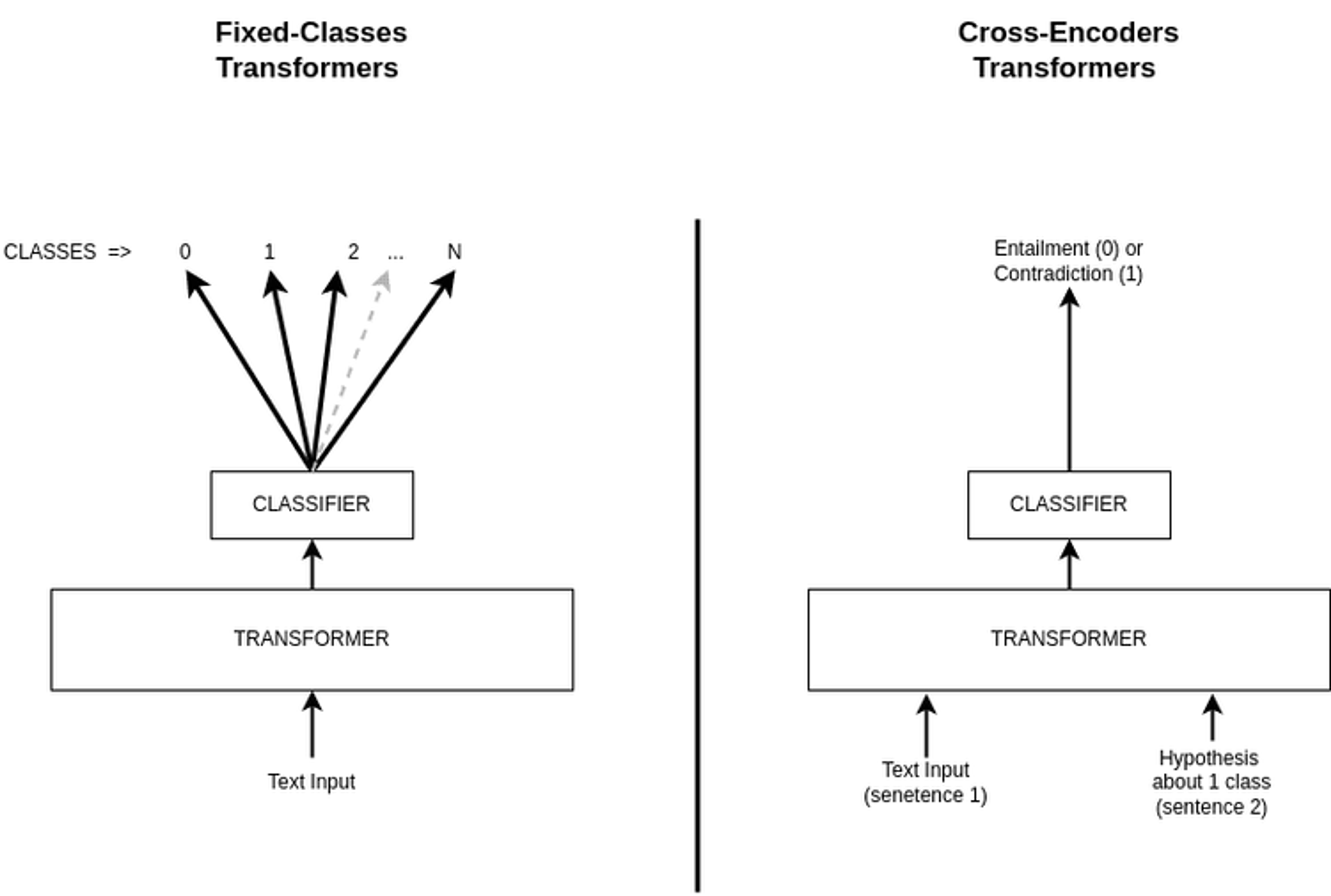
Cross-encoder architecture

Our label hierarchy is constantly evolving to accommodate a growing range of use-cases across our customer-base without sacrificing generality that our model didn’t see during training. For that reason, training a transformer model with a classification head and a fixed number of classes might be problematic. Indeed, this architecture is rigid and we have to retrain the model if we want to infer new classes. One of the solutions would be to use a cross-encoder architecture to transform the N-classes classification problem into a binary classification problem. This approach enables us to infer new classes without having to retrain the model.‍

However, by their architecture, cross-encoders have a “slow” forward pass because they can process only 2 sentences at a time. When we have a lot of samples and/or classes to train/infer on, it is computationally expensive to infer each possible class individually (even with batching).

Parallelized cross-encoders architecture via attention masking

With a few of my fellow Ntropians, we came up with an idea to parallelize the cross-encoders computations by forwarding not only two sentences (the input and the queried label) but multiple sentences (the input along with several labels) at once.

On the original cross encoders, an input like that would make no sense because the attention happens between each possible pair of input tokens. It means that each label would be dependent on the other labels and the output logits would depend on them also. For example, if we would add a single label to the input, it could change the value of the other logits. We don’t want that to happen.

We want each output logit to be dependent only on the text input, the hypothesis and his corresponding label input. The other label inputs should have no effect and we should have the same number of output logits as the number of input labels.

To make the output logits dependent only on their respective labels, we make use of a special attention mask to disable computation between specific tokens:

• The attention happens normally where each token attend to each other for each component of the input independently (text input, label 1, label 2, …, label N) (2-way attention)
• Each label’s token attends to the text input tokens (1-way attention)

Attention masking implementation

In order to have a custom attention mechanism like the one described above, we had to make some changes to the models (BERT and BART) of the HuggingFace transformers library. The main changes happen by using the 3 helper functions.

Those helper functions are applied directly to a batch with PyTorch vectorized operations:

• Input Segmentation

• Positional encoding

• Attention mask

These functions can be found on the GitHub repository, here.

Note that even the custom attention mask returned by the function above , is quite sparse as a lot of attention links have been removed (labels tokens ⇒ text input tokens).

Once we got this attention mask computed, we can just apply it before the attention layers. On the transformer’s output, we retrieve the logits scores from the [CLS] tokens’ positions.

Fewer layers in transformers

One extra technique that we use to get faster models, is to shrink the layers of the transformers. Indeed, for a lot of tasks/datasets, we realized that removing part of the layers would give no drop in performance while making the computation faster.

Here is a code snippet that keeps only the 2 first pre-trained layers of the Bert model (instead of 12).

Labels packing

During training, for each example, we sample N random negative labels plus the positive label. So for each example, the model is asked to make predictions on the true label and N false labels. Note that we have to keep a consistent number of labels per sample to be able to batch them together.

For the HuggingFace tokenizer, we always make use of the parameter `truncation=”only_first”` so that even if we have a long list of labels to infer, we will truncate the text input and not the labels input. Truncation at the end of the sequence would raise an error for any sequence longer than the model’s max length parameter.

During inference, for each sample, we generally want to infer all the possible labels. We set a “number of labels per sample” and loop over the list of all possible labels to get every label output score. If the “number of labels per sample” is not a multiple of the total number of labels, we pad the labels to keep consistency in the batches.

For example, let’s say we have:

• 6 labels to predict: [A, B, C, D, E, F]
• An input sentence: “Ant colony hits Australia”.

If we set the “number of labels per sample” parameter to 3, we would have the following two formatted input samples:

Ant colony hits Australia [SEP] This example is about [CLS] A [CLS] B [CLS] C

Ant colony hits Australia [SEP] This example is about [CLS] D [CLS] E [CLS] F

Now, with “number of labels per sample” = 4, we end up with two padded labels (“None”):

Ant colony hits Australia [SEP] This example is about [CLS] A [CLS] B [CLS] C [CLS] D

Ant colony hits Australia [SEP] This example is about [CLS] E [CLS] F [CLS] None [CLS] None

Of course, the less padded labels we have, the more optimized the inference will be.

Benchmark

To evaluate the performance gain of this approach, we chose a public text classification dataset, AG News (News text with 4 classes).

For the backbone model, we chose a DistilBart model with two layers in the encoder and one layer in the decoder.

Train time reduction

• Using a vanilla cross-encoder (one label per sample), an epoch takes more than 22 minutes.
• Using a parallelized multi-label cross-encoder (4/all labels per sample), an epoch takes around 2 minutes and 30 seconds.

It’s more than a 8x speedup for training time.

Test time reduction

• Using a vanilla cross-encoder, it takes 28.15 seconds to infer the full test set (F1 0.938)
• Using a parallelized multi-label cross-encoder, it takes only 10 seconds to infer the full test set when inferring with 4 labels per sample (F1 0.941)

Almost a 3x speedup for inference time without sacrificing the model’s accuracy.

Note that the more we have labels per sample the faster the inference is. Indeed the speedup can be even greater on a dataset where we have a high number of classes (got a 10x speedup on a private dataset using 32 labels per sample).

Conclusion

In this post, we presented a technique to make cross-encoders faster by just making few changes on the input formatting and the attention mask. On the AG News dataset (4 classes), training is 8 times faster and inference is 3 times faster when using the technique.

You can access the full implementation on this public GitHub repository.

If this sounds interesting and you want to learn more, feel free to shoot us a message. We’re hiring!